Welcome to U19960 --- Data Recovery and Analysis
This lab material accompanies your lectures for this module. Please use the navigation bar on the left to select the lab material you want to view.
Lab material will be release on a weekly basis.
| To quickly access these labs on your mobile phone or tablet, simply scan the QR code. |  |
Accessibility and Navigation
There are several methods for navigating through the chapters (i.e., sessions), and pages.
The pagetoc-bar on the right provides a list of sections in the currently opened page. You can click on each entry to quickly jump between sections and subsections. This is particularly useful if the page is very long and scrolling up and down is annoying.
The sidebar on the left provides a list of all chapters/sessions. Clicking on any of the chapter/session titles will load that page.
The sidebar may not automatically appear if the window is too narrow, particularly on mobile displays. In that situation, the menu icon () at the top-left of the page can be pressed to open and close the sidebar.
The arrow buttons at the bottom of the page can be used to navigate to the previous or the next chapter.
The left and right arrow keys on the keyboard can be used to navigate to the previous or the next chapter.
Top menu bar
The menu bar at the top of the page provides some icons for interacting with the book. The icons displayed will depend on the settings of how the book was generated.
| Icon | Description |
|---|---|
| Opens and closes the chapter listing sidebar. | |
| Opens a picker to choose a different color theme. | |
| Opens a search bar for searching within the book. | |
| Instructs the web browser to print the entire book. | |
| Opens a link to the website that hosts the source code of the book. | |
| Opens a page to directly edit the source of the page you are currently reading. |
Tapping the menu bar will scroll the page to the top.
Search
Each book has a built-in search system.
Pressing the search icon () in the menu bar, or pressing the S key on the keyboard will open an input box for entering search terms.
Typing some terms will show matching chapters and sections in real time.
Clicking any of the results will jump to that section. The up and down arrow keys can be used to navigate the results, and enter will open the highlighted section.
After loading a search result, the matching search terms will be highlighted in the text.
Clicking a highlighted word or pressing the Esc key will remove the highlighting.
You have the ability to change the theme of the mdBook by clicking the icon on the top left mdBook. Additionally, there is a toggle for the table of content, and a search tool.
Session 01
Basic Linux CLI (command-line interface) commands
A prompt is something a CLI will display to show the user that it's ready to receive input. Prompts come in all sizes, colours, shapes and forms depending on the shell an distribution you are using.
For example, your prompt might look like this: user@mymachine:~$
Or it might look minimalistic, like this: ~>
There are many ways a prompt can look, so for this reason the $ sign is used as a generic symbol in documentation and teaching to simply denote a prompt. And the commands after it are the ones you'll type (so don't type the $ at the beginning).
Do not copy-paste commands. You will notice that if you hover over the example command with your mouse, you'll get a symbol show up that allows you to copy the command into your clipboard, which you could paste into your terminal instead of typing it yourself. There are many reasons why this is a bad idea, generally. But specifically for these exercises, you'd be copy-pasting the $ symbol with the command, and when you try to execute the command you'll receive an error. More importantly though, from experience, I can promise you that typing in the commands by hand will help you learn them faster. Remember, using the CLI allows you to express yourself, or "talk" to the system.
What do the following commands do?
Use the man command, followed by the command you're interested in (see above example) to find out what it does. Note that not all commands have an accompanying manual page.
| Command | Command | Command | Command |
|---|---|---|---|
date | who | w | whoami |
echo | uname | passwd | ls |
ln | more | wc | cp |
mv | rm | find | chmod |
diff | head | tail | lpr |
which | gzip | gunzip | tar |
cd | pwd | mkdir | rmdir |
Alternatively, most commands can also be called with the optional argument --help, which will give you a brief (and sometimes not so brief) summary of how the command syntax works.
Directory Structure Exercise 1
Use the appropriate Linux command(s) to create the following directory tree in your home directory
graph TD;
  FileTypes --> TextFiles --> ShellScripts
  FileTypes --> BinaryFiles --> Byte-Code --> J-Code
                                Byte-Code --> P-Code
  FileTypes --> PostScriptFiles --> PDF
Directory Structure Exercise 2
Create the following list of files in a directory called LinuxEx2:
The first column of this table (and sometimes others) with the
#heading is simply there for orientation purposes; to help you keep track of which line you are on, and help you get back in case you have to interrupt or get otherwise distracted.
| # | Filename |
|---|---|
| 01 | Feb-99 |
| 02 | jan12.99 |
| 03 | jan19.99 |
| 04 | jan26.02 |
| 05 | jan5.99 |
| 06 | Jan-01 |
| 07 | Jan-98 |
| 08 | Jan-99 |
| 09 | Jan-00 |
| 10 | Mar-98 |
| 11 | memo1 |
| 12 | memo10 |
| 13 | memo2 |
| 14 | memo2.txt |
Explain what the following commands do
Experiment by executing these commands. Document what the output is and, in your own words, try to explain what the commands do. Write your observations down, either on paper or wherever you keep your lecture notes.
| # | Command to execute |
|---|---|
| 01 | echo * |
| 02 | echo jan* |
| 03 | echo M[a-df-z]* |
| 04 | echo ???? |
| 05 | echo ????? |
| 06 | echo *[0-9] |
| 07 | echo *[[:upper:]] |
| 08 | echo *.* |
| 09 | echo *99 |
| 10 | echo [FJM][ae][bnr]* |
| 11 | echo ls | wc -l |
| 12 | who | wc -l |
| 13 | ls *.txt | wc -l |
| 14 | who | sort |
| 15 | cp memo1 .. |
| 16 | rm ??? |
| 17 | mv memo2 memo2002 |
| 18 | rm *.txt |
| 19 | cd; pwd |
| 20 | sillycommand 2> errors |
A small script with nano
Change your working directory to your home directory. Start the nano text editor and type the text that follows. Then save this to a file called FirstTypedScript.sh:
#!/bin/env bash
#
# my first typed script
#

echo "Knowledge is Power"

#
# Two more commands.
#

# This one has an interesting optional argument
ls -R1

# This one is new
cat FirstTypedScript.sh

# Look this one up. Useful in shell scripts, like this one. Not much used in everyday CLI usage though.
exit 0
Checking and move FirstTypedScript.sh
Check that the newly created file exists in your home directory. Now move the file with the appropriate command(s) to the directory you created earlier, named ShellScripts.
What was that in the script?
Find out what the commands written in the FirstTypedScript.sh file do by typing them in manually on the prompt. Use the manual pages to help you discover more about each command (and optional arguments).
Wrapping it all up
Finally, run your first typed shell script by calling it:
$ ./FirstTypedScript.sh
What happens when you do this? Try finding a way of running the shell script.
Session 02
Click on a lab below:
Understanding Data
You are encouraged not to use a calculator to do the conversion.
- First use the reverse conversion to check your results.
- Finally, use the calculator only to check your results!
- This is "bread and butter" stuff. Do not skip it!
Position Coefficients
Write out each of the following numbers in the position coefficient format:
| # | |
|---|---|
| 1 | $$\mathtt{120_{10}}$$ |
| 2 | $$\mathtt{6482_{10}}$$ |
| 3 | $$\mathtt{1AF_{16}}$$ |
| 4 | $$\mathtt{9434_{16}}$$ |
| 5 | $$\mathtt{1100_{2}}$$ |
| 6 | $$\mathtt{10000011_{2}}$$ |
| 7 | $$\mathtt{11110000_{2}}$$ |
| 8 | $$\mathtt{345_{10}}$$ |
| 9 | $$\mathtt{1003_{10}}$$ |
| 10 | $$\mathtt{123_{16}}$$ |
| 11 | $$\mathtt{44AF_{16}}$$ |
| 12 | $$\mathtt{10100001_{2}}$$ |
Binary to Decimal Conversion
Convert the following from Binary to Decimal:
| # | Binary |
|---|---|
| 1 | $$\mathtt{11110000_{2}}$$ |
| 2 | $$\mathtt{11110001_{2}}$$ |
| 3 | $$\mathtt{01110000_{2}}$$ |
| 4 | $$\mathtt{00110001_{2}}$$ |
| 5 | $$\mathtt{10101010_{2}}$$ |
| 6 | $$\mathtt{10010000_{2}}$$ |
Binary to Hexadecimal Conversion
Convert the following from Binary to Hexadecimal:
| # | Binary |
|---|---|
| 1 | $$\mathtt{11110011_{2}}$$ |
| 2 | $$\mathtt{10010001_{2}}$$ |
| 3 | $$\mathtt{11010100_{2}}$$ |
| 4 | $$\mathtt{10111101_{2}}$$ |
| 5 | $$\mathtt{11101010_{2}}$$ |
| 6 | $$\mathtt{10010111_{2}}$$ |
Hexadecimal to Decimal Conversion
Convert the following from Hexadecimal to Denary
| # | Hexadecimal |
|---|---|
| 1 | $$\mathtt{AFAE_{16}}$$ |
| 2 | $$\mathtt{E0F1_{16}}$$ |
| 3 | $$\mathtt{C12D_{16}}$$ |
| 4* | $$\mathtt{F0CEF_{16}}$$ |
| 5* | $$\mathtt{C0FFEE_{16}}$$ |
| 6* | $$\mathtt{DEADBEEF_{16}}$$ |
All starred (*) numbers are a bit over the top, but you are welcome to try anyway, just be aware that they are pretty large decimal numbers!
ASCII Representations
What you'll need:
- A text editor (anything simple like Notepad will do)
- A hex editor, there are plenty for all operating systems, but here are a few:
- Get used to writing notes in investigations (and exercises), so make sure you have pen and paper or an easy electronic mean to record notes
Create a Plaintext ASCII File
- Open your text editor of choice (don't use Word or similar!)
- Write the following exactly as you see it here (substitute the YY for the current year) and save the file when done:
Hello Friend!

The year ends on every 31st of December. This year it'll be on 31/12/YY.
It's tempting, but don't make use of the copy-paste function when you hover your mouse over the above text. These convenience functions can introduce hidden characters that you can't see with your eyes, but will copy them into you editor anyway, and therefore might result in your file being different than intended for this exercise.
Explore the File and Editor
- Locate the file you just created and find out the file's size in bytes
- Start your editor of choice and figure out how to load the file you created just now
- Depending on your editor, you will usually see a view that is split in two, can you identify which side shows what?
Offset
The left most column (in all hex editors) shows the offset of the data.
- Try to figure out how offsets work (it might not always be obvious)
- If you're stuck, signal your tutor
Offsets are often written as 0xNN where NN is a number. For example, the beginning of the file loaded will be 0x00, the last should be 0x57.
- Can you figure out how I've arrived at
0x57?
Columns are as important as rows in determining the offset! And remember, we generally start counting from 0 in computing.
Locating Data
-
Locate
H, fromHello World, so first character- Note down the hex value for the character
- Note down the offset for the character
-
Locate
!- Note down the hex value for the character
- Note down the offset for the character
-
Locate
y, from the second occurrence ofyear- Note down the hex value for the character
- Note down the offset for the character
-
Count the bytes in the file. Does it match the size you identified earlier?
-
Find out what
Unicodeis, particularlyUTF-8andUTF-16(we'll encounter and discuss those as we move through module material)- What's the difference to ASCII?
Windows Registry
DO NOT CHANGE ANYTHING IN THE REGISTRY IF YOU DON'T KNOW WHAT YOU'RE DOING, YOU MIGHT END UP DOING IRREPARABLE DAMAGE TO WINDOWS!
The material you're going through here is designed to get you simply acquainted with some (but not all) artefacts found in the Windows registry. Later on in the module, you will be doing more in-depth analysis using specialist tools, such as Autopsy. Having advanced knowledge, then, of what is available in the Windows registry and what is of investigative value, will prove useful.
To access your Windows registry (ideally on your own PC rather than campus PCs), you'll need to execute regedit.exe. You can do this a few different ways:
- Hit the Windows-logo key on your keyboard, and just start typing
regedit, launch the found application with elevated privileges ("Run as administrator") - Open a Windows command prompt (
cmd), by following the same procedure in 1. above to elevate your privileges, then typeregeditto start the application
On campus machines, you might not be able to launch regedit with elevated privileges. If the method in 1. above doesn't work, try the second method in 2. without trying to elevate your privileges. You should be able to at least look at the registry.
- Go through each hive
- Expand each hive and explore keys and subkeys
- Locate the hive
HKEY_CURRENT_USER - Locate
Softwarewhich should give you a list of all the installed software - Drill down into each software listed and have a look if there are any differences
Windows MRU
Microsoft of course tries to make the use of Windows as comfortable as possible for their customers, so they always add a bunch of convenience functions into their products. On Windows, one of the earlier advancements was the introduction of the Most Recently Used (MRU) files and folders. The concept is simple, Windows remembers what you had accessed a while back so that when you want to find what you were working on, you'll get there faster.
Of course, this information is also very useful in investigations. If you have MRU active (which should be the case by default), you'll find the registry key here: HKEY_CURRENT_USER\Software\Microsoft\Windows\CurrentVersion\Explorer\RecentDocs
You should see something similar to this:
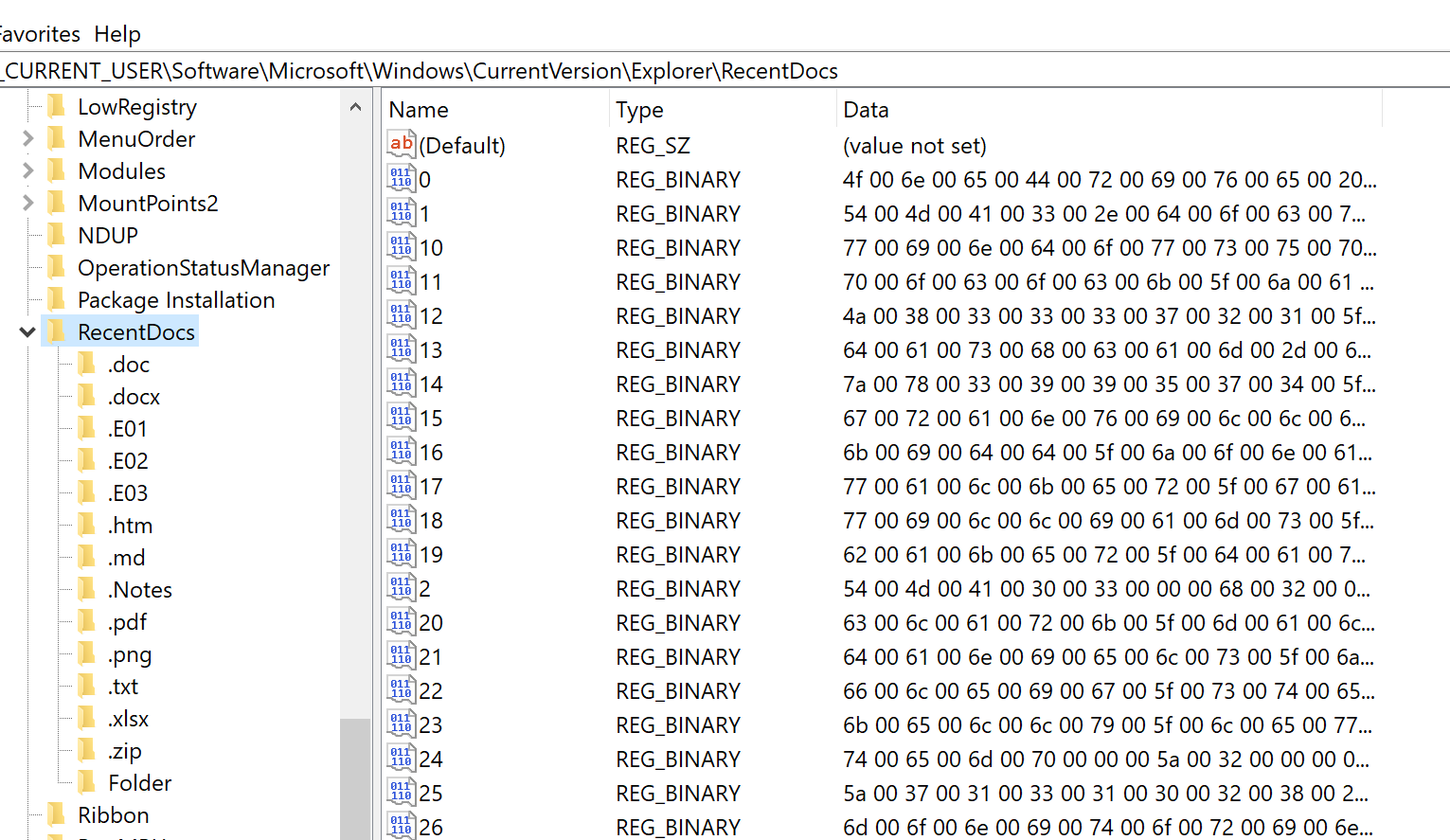
If, like in the screenshot, you've expanded the RecentDocs tree, you'll notice that there are is a bunch of hex encoded information associated with each entry in the right pane. When you double-click on an entry, you'll be presented with an editor that shows you the hex, and the ASCII equivalent, to the right. That's also where you'll find which file this entry is pointing to.
Jump Lists
Continuing the theme of convenience for Microsoft's customers, we also have Jump Lists at our disposal. Jump Lists are also on by default, and are particularly useful because they store per-user information on opened documents.
In digital forensics (or any forensics), you want to be able to attribute certain events to the person being investigated (or show that there is no attribution). For that, you'll want to collect as much meaningful evidence as possible. Certain artefacts carry more weight than others. Jump Lists have a lot of weight but, of course, they can't prove 100% that a user carried out a certain activity. Nonetheless, they provide a strong indicator.
Jump lists also come in two flavours: automatic and custom. The former are created during the user's everyday actions on the system, and the latter are created when a user pins a file to either the Start Menu or the Task Bar.
You can check your Jump List files using Windows Explorer (remember to turn on "Hidden Files"): C:\Users\yourUserName\AppData\Roaming\Microsoft\Windows\Recent Items\
Windows UserAssist Settings
This feature is very useful, particularly because it keeps track of which applications have been executed by a user. By default, it should have recorded your activity in your registry (unless you've turned it off).
- Open
regedit - Click on
Computerto make sure you've highlighted the root of the hive tree - Click on "Edit" and then "Find...", or hit CTRL+f
- Type
UserAssistin the search box - Ensure only
KeysandMatch whole string onlyare ticked - Click on
Find Next
There are a number of UserAssist entries present in the registry. Pay attention (and take notes) on which ones you found. Start exploring the entries, and you'll probably notice that some entries of Type REG_BINARY look weird.
Can you figure out why?
Windows Time Zone Settings
This setting is very crucial to investigators, as you can probably imagine. The main focus, of course, is ensuring that all timestamps on the system are interpreted correctly.
- Open
regedit - Navigate to
Computer\HKEY_LOCAL_MACHINE\SYSTEM\ControlSet001\Control\TimeZoneInformation
You'll see details that are important to an investigation. As you've now refreshed your understanding of hexadecimal, and binary, the data stored with each setting should not be difficult for you to decode.
Particularly of interest are:
ActiveTimeBiasBiasDaylightBias
ActiveTimeBias
It doesn't matter if daylight saving is being observed or not, this value holds the current time difference, in minutes, between local time and UTC, and therefore helps establish the current time zone.
Bias
This value holds the normal difference from UTC in minutes when daylight saving is not observed. If the system is set to UK time, then this value will usually be zero due to the UK residing in the GMT time zone. What this value holds, when not zero, is therefore the number of minutes that would need to be added to the local time to arrive at UTC time.
DaylightBias
This value, when daylight saving is observed, specifies by how much the local time should be adjusted to arrive at the local time that doesn't include daylight saving. This value is added to the value of the Bias member to form the bias used during daylight time. In most time zones the value of this member is -60 (converted from 0xFFFFFF4C and applying two's complement).
It is calculated based on the values of the StandardBias, DaylightBias, and Bias values, and if StandardBias (which is zero in most time zones) is used.
When Daylight Saving Time (DST) is being observed, the calculation is: ActiveTimeBias = Bias + DaylightBias
When DST is not observed, the calculation is: ActiveTimeBias = Bias + StandardBias
UTC, local time, and ActiveTimeBias can also be used for converting between local time and UTC, for example:
- UTC = local time +
ActiveTimeBias - local time = UTC -
ActiveTimeBias
And, of course, ActiveTimeBias can be calculated using UTC and local time:
ActiveTimeBias= UTC - local time
DaylightName
This value is used by Windows to show the current time zone setting.
DaylightStart
This value is used by Windows to record when daylight saving will come into force for the time zone the system is configured in.
StandardName
This value holds the current time zone setting when daylight saving is not active.
StandardStart
This value holds when standard time will commence in the time zone the system is configured in.
DynamicDaylightTimeDisabled
This is a boolean value that indicates if daylight saving is applied.
TimeZoneKeyName
Which time zone is configured can, depending on the version of Windows, also be read from this value. This value also takes precedence over StandardName, so if you're ever confronted with values in StandardName and this one, this one should be used, otherwise StandardName should be used.
Dynamic DST
This value depends on which timezone the machine is in. It's designed for those edge cases where some countries start observing daylight on a different day of the year.
Session 03
Problem Based Learning Lab - Sandboxie
Background
At 00:05 on the 12th September 2019 Vladimir NAVALNY, a high ranking member of the Russian Glavnoje Razvedyvatel'noje Upravlenije (GRU), was arrested in a joint operation with the National Crime Agency (NCA) and Kent Police at the port of Dover in Kent whilst attempting to enter the country arriving from Russia posing as a journalist under the false identity of Viktor YELTSIN. He had in his possession a forged passport (Exhibit DW/1), an iPhone 6S mobile phone (Exhibit DW/2), a laptop computer, believed to be running Windows 10 (DW/3) and €20,000 (Exhibit DW/4). Intelligence indicates that NAVALNY was attempting to meet with a contact in the UK Power network (Michael JAMES) and pass a specially developed virus, reportedly capable of taking down two thirds of the UK’s power network. During initial interview NAVALNY stated that the laptop was not his and that he was taking it to the UK for a friend to pass to JAMES. When asked to account for the €20,000, NAVALNY replied with no comment.
Intelligence also indicates that NAVALNY was using specialist software called "Sandboxie" to obfuscate his activities and that he may have removed all or part of this software from the laptop prior to travel to the UK.
Task Description
- Identify and explain the threats to an investigation posed by the use of Sandboxie software.
- Explain how the software operates in a form suitable for a court
- Considering the entire lifecycle of software on a computer, where might you look for evidence that software is or was located on a Windows computer?
- In light of this, how might you apply this to the laptop computer (DW/3)?
- What challenges might you expect to face in testing such software, and how might these be addressed?
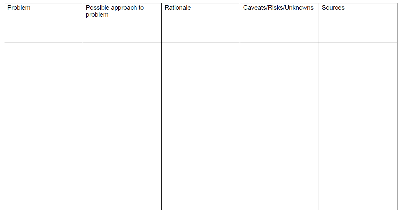
For each question above, record the things you do not know (the problems) on the table further down this page, along with your approach to solving the problem and your rationale.
Applying Lessons from PBL to Deployment
In this section, you will test out your theory and try to identify the relevant artefacts and understand their meaning.
- Deploy solution - investigate digital artefacts associated with the Sandboxie product. You may need to download this onto a USB and transfer it to your forensic PC1 see also2
- On completion of your analysis, produce a summary analysis note in the format seen in table 1 below
- Each group briefly presents problems identified from practice and suggested approaches (see table 2 below)
Table 1: Summary Analysis Note Template
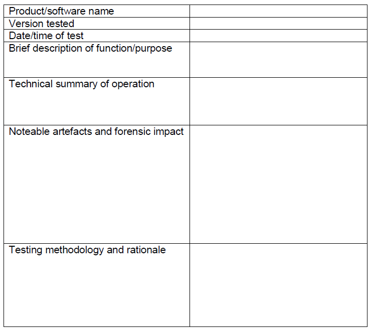
Table 2: Suggested PBL Template
-
Before you install the software, be sure to write down and discuss your proposed methodology for studying how the software works --- consider the entire lifecycle! ↩
-
Take notes throughout the process --- think ACPO Guidelines!! ↩
Session 04
Nothing to see here.
Session 05
Required resources:
HunterXP_100.raw(MD5: 3D74EB17210F40F03B5FC5C1937927D6) (available on Blackboard)Rajewski_GPT2_100.raw(MD5: 172C1D63EE78E293C66F1045C864E1FB) (available on Blackboard)- HxD (https://mh-nexus.de/en/hxd/) (Windows only)
Task 1: Decoding the MBR
Start HxD and under the menu Tools, open the disk image HunterXP_100.raw (Note: this file is only the first 100 sectors)
Asking HxD to open the file as a disk image will make it prompt you for the sector size, which in this case is the (usual) default of 512 bytes.
HxD can therefore help a bit by adding sector markers on the right-hand side of the "Decoded text" view, which will make it easier for you to see where one sector starts, and the other ends.
Now use your notes and the slide deck from Session 05 to answer the following:
1. How many entries are in the partition table?
Click to reveal answer
2. Which partition, if any, is configured to boot on start-up?
Click to reveal answer
3. Explain how you determined your answer to 2
Click to reveal answer
4. What file system would you expect to find in Partition 1?
Click to reveal answer
5. Explain how you determined your answer to 4
Click to reveal answer
6. What is the offset in bytes to the start of Partition 1?
Click to reveal answer
7. Explain how you determined your answer to 6
Click to reveal answer
8. Use the Search menu to go to the offset you found in 6 and mind the number system to enter the offset
9. Write down the first EIGHT hex values you should see.
Click to reveal answer
10. Starting with the first byte at the offset you identified in 6, highlight 1 sector's worth of bytes (click-n-drag)
11. What TWO similarities do you see in the highlighted sector compared to the MBR?
Click to reveal answer
Task 2: Decoding the GPT
Start HxD and under the menu Tools, open the disk image Rajewski_GPT2_100.raw (again, only the first 100 sectors)
Now use your notes and slide deck from Session 05 to answer the following questions.
1. How many entries are in the partition table?
Click to reveal answer
2. Explain how you determined your answer to 1 above
Click to reveal answer
3. For each partition you identified in 1, complete the table below
| GUID (hex values as stored) | GUID (hex values in human-readable form) |
|---|---|
| A2A... | EBD... |
| ... | ... |
| ... | ... |
| ... | ... |
Click to reveal answer
A2A0D0EBE5B9334487C068B6B72699C7 | EBD0A0A2-B9E5-4433-87C0-68B6B72699C7
A2A0D0EBE5B9334487C068B6B72699C7 | EBD0A0A2-B9E5-4433-87C0-68B6B72699C7
A2A0D0EBE5B9334487C068B6B72699C7 | EBD0A0A2-B9E5-4433-87C0-68B6B72699C7
Yes, all four have the same GUID but, for an investigator, it's important to note this down.
4. In the space below, add the partition information for the partitions you listed in Step 3
| Partition type | Size in MiB (Mebibytes) | Partition name |
|---|---|---|
| Basic... | ??? | Basic... |
Click to reveal answer
| Partition Type | Size in MiB (Mebibytes) | Partition Name |
|---|---|---|
| Basic Data Partition (Win) | 200 | Basic Data Partition |
| Basic Data Partition (Win) | 191 | FAT_VOLUME |
| Basic Data Partition (Win) | 191 | FAT2_VOLUME |
| Basic Data Partition (Win) | 191 | FAT3_VOLUME |
5. Show how you calculated the size of each partition listed above
Click to reveal answer
| First |
Last | Number of sectors (Last - First + 1) | Size (NumSectors * 512) | |
|---|---|---|---|---|
| 1 |
128 | 409727 | 409600 | 200 MiB |
| 2 | 509952 | 901119 | 391168 | 191 MiB |
| 3 |
901120 | 1292287 | 391168 |
191 MiB |
| 4 | 1294336 | 168503 | 391168 | 191 MiB |
Session 06
Click on a lab below:
Session 06 - FAT Filesystem
Requirements:
FAT16USB.img(MD5: D4EAEE279402DE18FD02C32975906053)HANDOUT-FAT16-Reference.pdf- A hex editor, for example HxD (https://www.mh-nexus.de/)
- Pen and paper (Nope, this is not a joke, to complete the lab, you'll have a much easier time using pen and paper to recreate the table information and then fill in your answers)
- Microsoft's "How FAT Works" documentation: https://learn.microsoft.com/en-us/previous-versions/windows/it-pro/windows-server-2003/cc776720(v=ws.10)
Task 1: Start your hex editor and load the forensic image
- If you're using HxD, then open the Tools menu and choose Open disk image...
- Check the MD5 hash of the image: (if you're on Linux, you know what to do), otherwise in HxD, select Analysis then Checksums, choose MD5 and click OK.
- Keep a record of the MD5 (remember, you should be doing this as part of your contemporaneous notes anyway).
- Does the hash match the one at the top of this document? Make a note if it does or doesn't.
Task 2: Analysis and interpretation of the FAT16 Reserved Area/Boot Sector
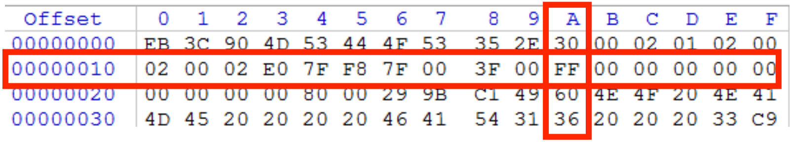
On using offsets: To find a hexadecimal offset, add the row offset to the column offset.
Example: Offset 0x1A would be the intersection of row 00000010, column A (as seen below, you'll find the value 0xFF).
- In which sector is the Boot sector located?
Click to reveal answer
- Use the handout (mentioned at the top of this document) and examine the sector you identified in 1 to complete the following table:
Hint: Make sure you reverse the byte order for values stored in more than 1 byte (recall: little-endian).
Table 1:
| Description | Offset (hex) | Length (bytes) | Value (decimal) |
|---|---|---|---|
| Bytes per sector | |||
| Sectors per cluster | |||
| No. of reserved sectors before FAT1 | |||
| No. of FAT tables | |||
| No. of sectors per FAT |
Click to reveal answer
| Description | Offset (hex) | Length (bytes) | Values (decimal) |
|---|---|---|---|
| Boot sector | 0x0B | 2 | 0x0200 = 512 |
| Sectors per cluster | 0x0D |
1 | 0x01 = 1 |
| No. of reserved sectors before FAT1 | 0x0E |
2 | 0x0002 = 2 |
| No. of FAT tables | 0x10 |
1 | 0x02 = 2 |
| No. of sectors per FAT | 0x16 |
2 | 0x0079 = 121 |
Task 3: Find the Root Directory and Data Regions
- Use your answers from Task 2 to calculate the offset from the start of the volume to the Root Directory using the following formula:
RDO (Root Directory Offset)
NRS (No. of Reserved Sectors before FAT1)
NFT (No. of FAT Tables)
SF  (Sectors per FAT)

RDO = NRS + (NFT * SF)
Click to reveal answer
- Enter the Root Directory Offset into the Sector box in HxD (if you're using another hex editor it should have similar functionality) to jump to that sector, as seen in the figure below.

- Use the handout to record the size of EACH directory entry in bytes. What size (in bytes) did you record?
Click to reveal answer
- The size of the Root Directory is found using the following formula:
RDS (Root Directory Size)
MNE (Max no. of Entries = 512)
SEE (Size of Each Entry)
NBS (No. of Bytes per Sector)

RDS = MNE * SEE / NBS
Use Table 1 and your answer from Task 3 to record the size of the Root Directory. What's the size (in sectors)?
Click to reveal answer
- Use your previous answers to determine the sectors for regions in the following Volume Map.
Hint: In the diagram and table, regions are marked with letters so it'll be easier to refer to them as you continue this exercise.
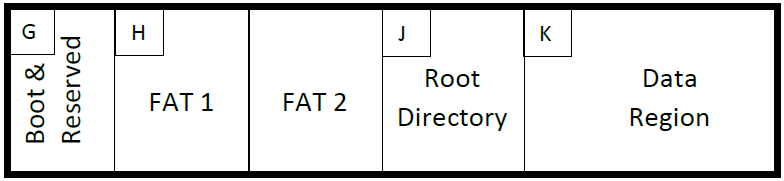
| Region | Answer |
|---|---|
| G | |
| H | |
| J | |
| K |
Click to reveal answer
| Region | Answer |
|---|---|
| G | 0 |
| H | 2 |
| J | 244 |
| K | 276 |
- What is the cluster number of the sector you identified in your answer above to the "K" region?
Hint: You may need to refer to your notes from class.
Click to reveal answer
Task 4: Find the starting cluster for each file
- Navigate to the sector where the Root Directory starts.
- Refresh your memory from Task 3 on the size of each directory entry (see your answer to Task 3.3).
- Starting at the top-left, highlight the number of bytes that you had to your answer to Task 3.3. (This is the FIRST directory entry).
- Locate the rows that begin with the filenames listed in Table 2 (Each row with a filename is the start of a directory entry).
- Use the handout to record in the table below the Directory Entry offsets, which map to the properties in Table 2.
| Description | Offset (hex)=(dec) | Size (bytes) |
|---|---|---|
| Extension | ||
| File size (bytes) | ||
| Starting cluster |
Click to reveal answer
| Description | Offset (hex)=(dec) | Size (bytes) |
|---|---|---|
| Extension | 0x08 = 8 | 3 |
| File size (bytes) | 0x1C = 28 | 4 |
| Starting Cluster | 0x1A = 26 | 2 |
- Remember: The offsets above are relative to the Directory Entry record.
- Use your answers above to complete Table 2 below.
| Filename | Extension | File size (bytes) | Starting Cluster |
|---|---|---|---|
| FILEA | |||
| FILEB | |||
| FILEC | |||
| FILED |
Click to reveal answer
| Filename | Extension | File size (bytes) | Starting Cluster |
|---|---|---|---|
| FILEA | TXT | "01 06 00 00" = 0x601 = 1537 | "03 00" = 0x0003 = 3 |
| FILEB | TXT | "00 02 00 00" = 0x200 = 512 | "07 00" = 0x0007 = 7 |
| FILEC | TXT | "FE 09 00 00" = 0x09FE = 2558 | "08 00" = 0x0008 = 8 |
| FILED | TXT | "32 0E 00 00" = 0x0E32 = 3634 | "0D 00" = 0x000D = 13 |
Task 5: Find the starting cluster for each file
- Start by completing this data region table by using your answers from above:
| Data region | Data |
|---|---|
| First Cluster | |
| First Sector | |
| Bytes per Cluster |
Click to reveal answer
| Data region | Data |
|---|---|
| First Cluster | 2 |
| First Sector | 276 |
| Bytes per Cluster | 512 |
- Go to the sector where FAT1 is located and complete the following table.
Hints:
- The start of the FAT entry is
F8 FF- FAT entries/clusters are numbered/counted from 0 in the FAT table
- Each FAT entry is 2 bytes long
Table 3:
| File name | Cluster chain (FAT entries) |
|---|---|
| File A | |
| File B | |
| File C | |
| File D |
Click to reveal answer
| Filename | Cluster Chain (FAT entries) |
|---|---|
| FILEA | 3 -> 4, 4 -> 5, 5 -> 6, 6 -> FFFF |
| FILEB | 7 -> FFFF |
| FILEC | 8 -> 9, 9 -> 10, 10 -> 11, 11 -> 12, 12 -> FFFF |
| FILED | 13 -> 14, 14 -> 15, 15 -> 16, 16 -> 17, 17 -> 18, 18 -> 19, 19 -> 20, 20 -> FFFF |
- Examine the content of each of the clusters in Table 3.
Is there anything unusual about any of these files? If so, record your observation and interpretation in your contemporaneous notes.
Click to reveal answer
Session 06 - Linux Tools
Requirements:
- A computer that runs Linux; OR
- A virtual machine that runs Linux
- A USB stick you don't care about any more and is rather small in storage capacity (the smaller the better, and make sure you've copied any important files off the USB stick onto somewhere else)
- The
Grundy_Tutorial.zipfile from Blackboard
Analysis Organisation
- Depending on your Linux distribution, you may have to find out how to deactivate auto-mounting of plugged in media (e.g., USB sticks)
- It's best to simply plug a USB stick into your machine first to find out if it is auto-mounted at all before you go looking for instructions
Note: As you've hopefully come across before, the
$shown in these example commands is simply a dummy placeholder for your prompt, which will look different from everyone else's prompt., so$is used generically. Of course, that means that you do not type the$.
You can use a few commands to figure out which device identifier your USB stick received after you plugged it in (e.g., /dev/sdb, /dev/sdc, etc.):
-
$ dmesg | tail(this will show you the last 10 lines of the system's log that will show you the device identification your USB stick received) -
$ dmesg | less(this will show you the full log which you can scroll up and down, useqto quit and return to your prompt)
DO NOT IGNORE THIS: The following might render your system unbootable if you get it wrong, so be very careful and only use a system that you're happy to re-install Linux onto. If you're doing this with a VM you'll have to ensure that you're passing the USB stick into the virtual machine (less risky). You have been warned!
Note: Most of the commands in this exercise require you, the user, to have elevated privileges. That means you'll have to execute them by prepending
sudo. For example:$ sudo wipefs -a ...
"Zeroing" a Disk
Zeroing a disk (or USB stick) means wiping it clean of any residue data that might have been there before you use it for this exercise. A bit like a real physical laboratory, you want to make sure that there is no residue that could interfere with your results.
The Correct but Impractical Way (for this exercise)
Due to modern disk (or USB stick) sizes this might not be feasible (1GB+ is going to take a while). The command will literally write 512-byte chunks of zeroes to your USB stick, and of course, the bigger your storage the longer it'll take. So, unless you really want to, don't do this command. It is here for documentation purposes, and so you know what you could do if you wanted to wipe a disk clean with zeroes.
$ dd if=/dev/zero of=/dev/sdX bs=512
(Note that X in /dev/sdX is just a placeholder here, and you will have to substitute it for the actual letter that the system gave the USB stick once you plugged it in, as mentioned at the start of this document)
Once the disk has been filled with zeroes, dd would terminate, and you could check that the disk is in fact full of zeroes by running:
$ xxd -a /dev/sdX
(again, same drive identifier as determined earlier)
The Less Correct but Practical Way (for this exercise)
Take the smallest USB stick you have, and make sure that you have copied any important data from it to a safe location, before attempting this.
The following only removes the partition information (MBR and GPT) but does not attempt to fill the disk with zeroes. Of course this is not very thorough and certainly not a secure way of wiping data (despite what the tool's name might insinuate).
$ wipefs -a /dev/sdX
Unzip the Grundy_Tutorial.zip File
First make sure that you're in your "home" directory (ensure that you do NOT prepend the following command with sudo):
$ cd ~
Double-check with the pwd command (ensure that you do NOT prepend the following command with sudo):
$ pwd
Your output should be something like this:
/home/user/
(where "user" is your username)
If you haven't done so already, move the Grundy_Tutorial.zip file from your "Downloads" directory to your home directory:
$ mv ~/Downloads/Grundy_Tutorial.zip ~
Now unzip the Grundy_Tutorial.zip file, for example:
$ unzip Grundy_Tutorial.zip -d Grundy_Tutorial
This will create a directory called Grundy_Tutorial, and inside you'll find the extracted contents. Make sure you changed directory to it:
$ cd Grundy_Tutorial
$ ls
The ls command should list the contents of the directory you're in now, and should show the following files:
able2.tar.gzimage_carve.rawlinuxintro-LEFE-2.55.pdflogs.tar.gzpractical.floppy.dd
If this is not the case, follow the above instructions from the top where you unzip the Grundy_Tutorial.zip file.
Copy the Floppy Image to a USB Stick
This will write the image, "as is" to the USB stick, ensure that you've double-checked that you're writing to the correct device that is associated with your USB stick (e.g., /dev/sdb, etc.)!!!
$ dd if=practical.floppy.dd of=/dev/sdX
(again, remember that sdX is just a placeholder for your actual drive identifier)
Now create a directory that you'll use to gather evidence:
$ mkdir evidence
Finally, create a directory that you'll use as a mount-point for the USB stick:
$ mkdir analysis
Determining the Structure of the Disk
Use lsblk to determine the disks your system can see. You should be able to find your USB stick's device identifier.
Get partition information from your USB stick:
$ fdisk -l /dev/sdX
Repeat that command, but this time save the output into a file for later:
$ fdisk -l /dev/sdX > ./evidence/fdisk.disk1
Creating a Forensic Image of the Suspect Disk
Change directory to evidence directory:
$ cd evidence
Take an image of the USB stick:
$ dd if=/dev/sdX of=image.dd bs=512
Change permissions on the image file to read-only:
$ chmod 444 image.dd
Mounting a Restored Image (via USB stick)
Change directory back to Grundy_Tutorial directory:
$ cd ..
Mount the USB stick:
$ mount -t vfat -o ro,noexec /dev/sdX ./analysis
Side-quest: Find out what the additional
-ooptionsnodevandnoatimewould do.
Change directory to analysis directory:
$ cd analysis
Have a look around (using cd and ls to navigate and list files and directories)
After you've completed your exploration make sure you're back in the Grundy_Tutorial directory:
$ cd ~/Grundy_Tutorial
Unmount the USB stick:
$ umount analysis
Mounting the Image File using the Loopback Device
We can also just mount the image directly, without having to go via a USB stick.
$ mount -t vfat -o ro,noexec,loop image.dd analysis
Question: Why does this work? Check the manual page for the
mountcommand and find what theloopoption does.
Change directory into the analysis directory once more.
$ cd analysis
Once more, explore.
When done, make sure you're back in the Grundy_Tutorial directory and unmount the image file:
$ umount analysis
File Hash
Let's create some hash sums next, which is the equivalent of a digital fingerprint.
Try sha1sum first to generate a hash for the USB stick:
$ sha1sum /dev/sdX
Now, try md5sum next, to do the same thing, but note the difference in hash length:
$ md5sum /dev/sdX
A good investigator always records their steps, so let's repeat that, but this time redirect the output into a file:
$ sha1sum /dev/sdX > ./evidence/usb.sha1sum
$ md5sum /dev/sdX > ./evidence/usb.md5sum
Let's now generate hashes from the files on the image file. Once again, mount the image file using the loopback device:
$ mount -t vfat -o ro,noexec,loop image.dd analysis
The following combination of commands will find regular files on the filesystem of the mounted image file and run a hash on each file it finds, it will then redirect the output and store it in a file list:
$ find ./analysis/ -type f -exec sha1sum {} \; > ./evidence/filelist.sha1sum
$ find ./analysis/ -type f -exec md5sum {} \; > ./evidence/filelist.md5sum
Have a look at the hashes:
$ cat ./evidence/filelist.*
Comparing all the hashes with your eyes is slow, tedious, annoying, and error-prone. So, let's have Linux check the hashes for us instead:
$ sha1sum -c ./evidence/filelist.sha1sum
(should return OK for each file if the file is unchanged)
Repeat the check for the MD5 hashes.
The Analysis
Remember each command can be output to a file using redirection. First, navigate through the directories:
$ ls -alR | less
(you can return to your prompt by pressing q for "quit")
Making a List of All Files (from the analysis directory)
For good measure, let's also create a list of all the files on the mounted image:
$ ls -laiRtu > ./evidence/listed_files.list
$ find ./analysis/ -type f > ./evidence/found_files.list
We also use the extracted file lists to find certain file names, for example those ending in jpg:
$ grep -i jpg ./evidence/found_files.list
Making a List of File Types
Let's find the filetypes (remember, file-extensions are meaningless in Linux-world, but can be (ab)used to confuse operating systems that rely on them to launch the appropriate application for the extension; such as Windows):
$ find ./analysis/ -type f -exec file {} \; > ./evidence/filetypes.list
Let's have a look:
$ cat ./evidence/filetypes.list
Now, let's see if we can find files that are not what they seem:
$ grep image ./evidence/filetypes.list
Can you see something that might be suspicious?
Viewing Files
We can also extract information from binary files (i.e., executables/compiled files) using a nifty little tool called strings:
$ strings ./analysis/arp.exe | less
(see if you can find the usage message)
Finally, unmount the image again:
$ umount ./analysis
And you're done!
Session 07
Requirements for the exercises in these sessions:
able2.tar.gz(Grundy's Tutorial)logs.tar.gz(Grundy's Tutorial)practical.floppy.dd(Grundy's Tutorial)image_carve.raw(Blackboard) (MD5: 3d76854d53317eee53b33258c3ac87f1)- A Linux distribution as a VM or bare-metal (e.g., Kali)
- Analysis of tarballed messages
- Splitting images
- Carving partitions with dd
- Carving a picture out of a junkfile with dd
Session 07 - Analysis of Tarballed Message Logs
Requirements are found here
Extracting a tar Archive
Assuming you're logged into your Linux machine, and you're in your home directory, change directory into your analysis directory (if you don't have it any more, create it with mkdir).
$ mkdir -p ~/analysis/logs
Ensure that you've transferred the logs.tar.gz file over to your machine and that the file lives in ~/analysis/logs.
Use the tar command to interact with tarballed files (they are archives that have had compression added to them, a bit like ZIP).
The tar command has a number of flags, such as:
t- list archive contentsz- decompress usinggunzipv- verbose outputf- apply actions to the file in question (e.g.,logs.tar.gz)
Let's first examine the content of the archive (here, we'll also be chaining the flags without each having a separate - prefix, this only works on some commands, such as tar):
$ tar -tzvf logs.tar.gz
What you should get back is an output of 5 log files (messages*), numbering from log rotation.
Does anything look dangerous? Once you've satisfied yourself, you can proceed to actually "untar" the archive:
$ tar xzvf logs.tar.gz
(as you might have already guessed, x stands for extract)
The 5 files you saw earlier should now be extracted in your current directory.
Look at one log entry from one of the files:
$ cat messages | head -n 1
(remember, if none of these commands mean anything to you, look them up with man)
Look at the format of the log files:
- Date
- Time
- Hostname
- Generating application
- Message
Analysing Messages
We want useful information, and the logs all have the same structure. So, we can concatenate them:
$ cat messages* | less
(press q if you want to exit less, you can use your up and down arrow keys to page/scroll through the buffer).
There's a problem, though. The dates ascend, then jump to an earlier date, then ascend again. This is because the later log entries are added to the bottom of each file, so as files are concatenated, the dates appear out of order.
We can fix that with the power of command pipes:
$ tac messages* | less
(not sure what tac does? Think about it, and look it up using man)
Let's Get Funky
We want to manipulate specific fields using awk. This command uses whitespace as its default field separator:
$ tac messages* | awk '{print $1" "$2}' | less
Sweet! Let's clean it up a bit, so we only have one entry per date:
$ tac messages* | awk '{print $1" "$2}' | uniq | less
(not sure what uniq does? Again, think about it, and look it up using man)
Nice. What about if we're interested in a particular date?
$ tac messages* | grep "Nov 4"`
$ tac messages* | grep ^"Nov 4"`
$ tac messages* | grep ^"Nov[ ]*4`
The more complex looking search strings are called "RegEx", short for "Regular Expressions", and they are very powerful ways of searching for data.
Now, let's check some suspect entries, e.g., "Did not receive identification string from
$ tac messages* | grep "identification string" | less
Let's say we just want date (f1&f2), time (f3) and remote IP (last field, $NF, number of fields)
$ tac messages* | grep "identification string" | awk '{print $1" "$2" "$3" "$NF}' | less
We can make that even neater by introducing the tab escape character \t.
$ tac messages* | grep "identification string" | awk '{print $1" "$2"\t"$3"\t"$NF}' | less
Report Time
We can use all of this to easily create a delicious looking report.
First, let's write a header:
$ echo "hostname123: Log entries from /var/log/messages" > report.txt
Now let's add what this part of the report is about:
$ echo "\"Did not receive identification string\":" >> report.txt
(the >> amends the already existing file, if you typed > then you've overwritten the previous message, so make sure you use >> to amend!)
Now let's add the actual information to the report:
$ tac messages* | grep "identification string" | awk '{print $1" "$2"\t"$3"\t"$NF}' >> report.txt
Let's continue by adding a sorted list of unique IP addresses, we start with the header information so we know what this part is about:
$ echo "Unique IP addresses:" >> report.txt
Now let's add the actual unique information:
$ tac messages* | grep "identification string" | awk '{print $NF}' | sort -u >> report.txt
BAM! Awesome. As you can probably already tell, this lends itself really well to be completely automated in, say, a script? You could feed this information into a script that then continues with some automation tasks, such as taking the IP addresses and putting them through nslookup and whois queries to get more details about the IP addresses.
Anyway, now have a look at your report, which should look like this:
$ less report.txt
```bash

```text
hostname123: LOg entries from /var/log/messages
"Did not receive identification string":
Nov     22      23:48:47        19x.xx9.220.35
Nov     22      23:48:47        19x.xx9.220.35
Nov     20      14:13:11        200.xx.114.131
Nov     18      18:55:06        6x.x2.248.243
Nov     17      19:26:43        200.xx.72.129
Nov     17      10:57:11        2xx.71.188.192
Nov     17      10:57:11        2xx.71.188.192
Nov     17      10:57:11        2xx.71.188.192
Nov     11      16:37:29        6x.x44.180.27
Nov     11      16:37:29        6x.x44.180.27
Nov     11      16:37:24        6x.x44.180.27
Nov     5       18:56:00        212.xx.13.130
Nov     5       18:56:00        212.xx.13.130
Nov     5       18:56:00        212.xx.13.130
Nov     3       01:52:31        2xx.54.67.197
Nov     3       01:52:01        2xx.54.67.197
Nov     3       01:52:00        2xx.54.67.197
Oct     31      16:11:17        xx.192.39.131
Oct     31      16:11:17        xx.192.39.131
Oct     31      16:11:17        xx.192.39.131
Oct     31      16:10:51        xx.192.39.131
Oct     31      16:10:51        xx.192.39.131
Oct     31      16:10:51        xx.192.39.131
Oct     27      12:40:26        2xx.x48.210.129
Oct     27      12:40:26        2xx.x48.210.129
Oct     27      12:40:26        2xx.x48.210.129
Oct     27      12:39:38        2xx.x48.210.129
Oct     27      12:39:37        2xx.x48.210.129
Oct     27      12:39:37        2xx.x48.210.129
Oct     27      12:39:14        2xx.x48.210.129
Oct     27      12:39:13        2xx.x48.210.129
Oct     27      12:39:13        2xx.x48.210.129
Oct     27      12:39:02        2xx.x48.210.129
Oct     27      12:39:01        2xx.x48.210.129
Oct     27      12:39:01        2xx.x48.210.129
Unique IP addressess:
19x.xx9.220.35
200.xx.114.131
200.xx.72.129
212.xx.13.130
2xx.54.67.197
2xx.71.188.192
2xx.x48.210.129
6x.x2.248.243
6x.x44.180.27
xx.192.39.131
Neat.
Technically, you could even save your command history up until now to record what you did and how you did it:
$ history -w history.txt
Which you then could feed into the beginnings of a script:
$ tail history.txt > reportmaker.sh
But that's for another time.
Session 07 - Splitting Images
Requirements are found here
Sometimes, and for various reasons, you might need to split big image files into smaller chunks. For example, if you're requested to supply the image file on multiple Blu-ray discs, or whatever. It happens. So, here's how to do that, albeit with a much smaller file.
As with the log files earlier, transfer the practical.floppy.dd to your machine, then create an appropriate directory:
$ mkdir -p ~/analysis/splitters
Move the file practical.floppy.dd to that directory. If you don't know how to move a file, go back through the labs, or look it up.
Hint:
mv
Now split the file into 360k chunks:
$ split -b 360k practical.floppy.dd image.split.
We could use split -d -b 360k practical.floppy.dd image.split. if a newer version of split is installed. -d gives decimal numbering.
Let's have a look at what split produced:
$ ls -l image.split.a*
Now, let's fuse them back together using the concatenate command, cat:
$ cat image.split.aa image.split.ab image.split.ac image.split.ad > image1.new
Bit annoying, so how about we try it like this:
$ cat image.split.* > image2.new
Double-check we have two extra image*.new files:
$ ls -l
Now, let's have Linux figure out if the fingerprints still match for the original file and the two newly fused files; technically there should be no difference, but we will only be able to tell after generating hash sums:
$ sha1sum image1.new image2.new practical.floppy.dd
And? If they are different, then you need to go back and double-check where you went wrong.
Let's do the same, but with dd
This could be used on a real block device (i.e., hard disk, CD, etc.).
$ dd if=practical.floppy.dd | split -b 360k - floppy.split.
Double-check we have our split files:
$ ls -l
Now check that split files would generate the same hashes if we were to concatenate them in memory:
$ cat floppy.split.a* | sha1sum
Looking good? Let's create a complete image out of the split files then:
$ cat floppy.split.a* > new.floppy.image
Double-check:
$ ls -lh
And, once again, verify the hash:
$ sha1sum new.floppy.image
In fact, let's check all splits and assembled files:
$ sha1sum *
Session 07 - Carving Partitions with dd
Requirements are found here
Make sure you've transferred able2.tar.gz to your machine, as usual, the home directory is a good place.
Start the Task
Create a directory to store the transferred able2.tar.gz file.
$ mkdir ~/analysis/able2
Move the able2.tar.gz file from your home directory into the able2 directory.
$ mv ~/able2.tar.gz ~/analysis/able2
Now change directory into that newly created directory.
$ cd ~/analysis/able2
Now extract able2.tar.gz.
$ tar -xzvf able2.tar.gz
List the contents of the able2 directory again to see if the files were extracted successfully.
$ ls -lh
When the forensic image file was created, the author helpfully also created an md5sum generated hash file. Have a look at its contents.
$ cat md5.dd
Make a note of the hash, or you could also have md5sum check it for you and inform you if the hashes match instead of you comparing this long sequence of numbers and letters manually with your eyeballs.
$ md5sum able2.dd
Better have this be done automatically.
$ md5sum -c md5.dd
The next command will give the output of what would have been an fdisk -l /dev/hdd and sfdisk -l -uS /dev/hdd. Scroll down to the sfdisk output/refer to output on page 76 of the Grundy tutorial file version 2.55.
$ less able2.log
Now it is time the image file is split into its various partitions which correspond to the information given in the log file.
$ dd if=able2.dd of=able2.part1.dd bs=512 skip=57 count=10203
$ dd if=able2.dd of=able2.part2.dd bs=512 skip=10260 count=102600
$ dd if=able2.dd of=able2.part3.dd bs=512 skip=112860 count=65835
$ dd if=able2.dd of=able2.part4.dd bs=512 skip=178695 count=496755
$ sfdisk -l -uS able2.dd
Session 07 - Carving a Picture out of a file with dd
Requirements are found here
This exercise is designed to teach you the very basics of hand-carving specific data from an image file, or directly from a damaged filesystem.
Settings things up
Additionally, ensure that your Linux distribution has the following tools installed:
First check if these tools are installed using which (e.g., $ which xxd and $ which bc, if you simply get your prompt back then they are not installed, if you get something back like /usr/bin/xxd, then you have them installed).
xxda hexdumperbca commandline calculator
How these tools must be installed depends on your distribution. If you're using a Debian-derived Linux distribution such as Ubuntu, Mint, or Kali, to name a few, then the following will install the above software using the apt package manager:
$ sudo apt update
$ sudo apt install xxd bc
If your Linux distribution is not based on Debian, find out which one it is based on and use the appropriate package manager for that distribution instead. The invocation will be very similar.
Make sure you've transferred the file
image_carve.rawto your machine.
Start the Task
Create a directory called carving, move the image file into it, and change into the directory.
$ mkdir -p ~/analysis/carving
Assuming you've saved the image_carve.raw file in your home, move it to the newly created directory.
$ mv ~/image_carve.raw ~/analysis/carving/
Change into the directory.
$ cd ~/analysis/carving
View image_carve.raw using xxd.
$ xxd image_carve.raw | less
Note: You'll see a bunch of random characters flying past your screen. Somewhere in there is a JPEG file.
The Concept
Conceptually, Figure 1 below should help visualise what our goal is:
 Figure 1: Conceptual diagram of a picture surrounded by junk data
The green represents "random" characters, which might be actually random data, or it might be another file, or it might be only part of another file. The yellow and red represents the JPEG file. The red parts indicate the header (ffd8) and trailer/footer (ffd9) of the JPEG.
Extraction Plan
Here's what you'll want to do:
- Find the start of the JPEG (using xxd and grep)
- Find the end of the JPEG (using xxd and grep)
- Calculate the size of the JPEG (in bytes using bc)
- Cut from the start to the end and output a file (using dd)
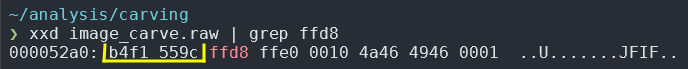
First Step
$ xxd image_carve.raw | grep ffd8
Note: You might recall, most files have header and footer information, JPEG's have
ffd8as their header identifier, andffd9as the footer.
You will see the offset 00052a0, which is the beginning of the line where ffd8 was found.
Note: The view is similar to what you're used to in
HxD, so row, and column - except thatxxddoesn't provide columns! (╯°□°)╯︵ ┻━┻
Second Step
Next, we must convert that offset to a number we can later pass on to dd (more later).
$ echo "ibase=16;000052A0" | bc
Note:
bccan't deal with lower-case letters, so you must make sure you remember to replace any lower-case letter with its upper-case equivalent!
This will return 21152 (same offset, just converted to decimal). The start of the JPEG, however, is actually 4 bytes further in, so we need to add 4 bytes to the current offset, which gives us a new offset of 21156, see the below image with yellow highlighting the 4 bytes that need to be added just before ffd8 starts.
Third Step
Now that we know where the beginning of the JPEG file is, we must find its end. To do that, we include the offset from earlier in the search (so we can avoid false-positive results):
$ xxd -s 21156 image_carve.raw | grep ffd9
This will return an offset in hex of 00006c74 as the beginning of the line containing ffd9.
Fourth Step
As before, we will also need to convert the footer offset from hex to decimal. We will need this information so we can calculate how big the JPEG is.
$ echo "ibase=16;0006C74" | bc
This will return 27764 (same offset, converted to decimal, as before).
We also need to include the remainder of ffd9. If we were to just carve up to ffd9 we would miss the entire footer which, forensically speaking, is not ideal. We can simply add 2 bytes to the offset in this case, and our result will be: 27766.

Fifth Step
With the adjusted offsets we found and calculated earlier, we can now calculate the size of the JPEG file, using simple arithmetic and the useful commandline calculator, bc.
$ echo "27766-21156" | bc
This will return 6610 bytes, which tells us how big the JPEG is.
Sixth Step
We have all the information we need to manually carve the JPEG from the image file.
$ dd if=image_carve.raw of=result.jpg skip=21156 bs=1 count=6610
The process will be really quick and if you now type ls to list your directory contents, you'll see a new file, result.jpg. Launch a command, or double-click on the file in your file manager, to view it.
You are encouraged to view the man page for dd to understand the commandline switches we used, but here's a quick breakdown:
| Switch | Description |
|---|---|
| if= | Input File, the file you want dd to work on |
| of= | Output File, the file name you want dd to write the result to |
| skip= | Skip n bytes into the input file before starting the extraction |
| bs= | The amount of bytes dd should read at once. By default dd uses 512 bytes, which is not precise enough for our purposes, so we set it to 1 |
| count= | This tells dd how many times dd should apply the bs= count from earlier |
If we were to leave bs= alone, the default of 512 bytes would apply, and subsequently dd would carve 512 * 6610 bytes, which is not what we want. We want dd to carve exactly 6610 bytes (as this is the size of the JPEG file), hence 1 * 6610.
Now What?
At some point soon, you'll receive instructions on how to create your own image file. You are in control of the contents of that image file, and therefore you'll be able to experiment with different file signatures (i.e. headers and footers/tails). This exercise used a very simple image file where the offsets are grouped (e.g., ffd9 vs ff d9). As you continue to experiment, you'll have to find ways of compensating for such discrepancies.
xxd has various commandline options that will, for example, change the count and width of displayed columns. Experiment with that if you are stuck and can't find your signature easily.
Session 08
Click on a lab below:
Session 08 - Sleuthkit
Requirements:
- A Linux machine
- Sleuthkit installed on the Linux machine
able2.ddfound inable2.tar.gz(Grundy's Tutorial)
Introduction
To complete this exercise you must ensure that you have transferred the able2.tar.gz to your forensic Virtual Machine (VM) or bare-metal machine.
Start the task
Note: Remember to create a directory where you can do focused work, for example
~/analysisin your home directory.
Display the image attributes including the type of image and the format.
$ img_stat able2.dd
To see what this looks like on an image that has been split, use the following command. Check the manual page for split to see what the flags -d -b do.
$ split -d -b 100m able2.dd able2.split.
Note: Yes, the dot at the end is intentional.
List the directory contents to check how many splits were created.
$ ls -lh able2.split.0*
Now re-check the image attributes, but this time on the split files.
$ img_stat able2.split.0*
We have seen that sfdisk is used to determine partition offsets within an image. Sleuthkit has mmls for this.
$ mmls -i raw -t dos able2.split.0*
The fsstat tool provides filesystem-specific information about the filesystem (the -o option gives us our offset which we can get from sfdisk or mmls).
$ fsstat -o 10260 able2.dd
The fls command lists the filenames and directories contained in a filesystem (-F file entries, -r descend into directories, -d display deleted entries). Please see the manual page for fls for more information.
$ fls -o 10260 -Frd able2.dd
Note: Remember that all of these commands could be appended to a report using redirect (
>>) to add the output of your commands to a log file.
It's important to remember that inodes are used to store metadata. This includes modified/accessed/changed (MAC) times and a list of all blocks allocated to a file. The following command will give you more information.
$ istat -o 10260 able2.dd 2139
The istat tool supports a number of filesystems. You should be aware of which filesystems it can handle, so you will want to list them.
$ istat -f list
It is time now to recover a deleted file. Having the inode information at the ready you can redirect the output of icat working on the referenced inode into a file.
$ icat -o 10260 able2.dd 2139 > lrkn.tgz.2139
What kind of file is this? Find out using the ever-useful file command.
$ file lrkn.tgz.2139
View the contents of the tarball archive.
$ tar -tvf lrkn.tgz.2139 | less
Instead of extracting the entire archive and then picking out the file that interests us (README file in this case), we can also simply send the contents of the file in the archive to stdout (using the O flag), which we then can redirect into a separate file.
$ tar -xvOf lrkn.tgz.2139 lrk3/README > README.2139
View the README.
$ less README.2139
And you're done!
Session 08 - Graphic Image Location and Display
Requirements:
- A Linux machine
- Sleuthkit installed on the Linux machine
practical.floppy.dd(Grundy's Tutorial)
Preparing for the Task
Create an analysis directory, and a mount sub-directory, unless you've already done so. Here we'll make use of the -p flag to create any missing sub-directories. If you get an error, then it's likely that you've already created these directories, so don't follow this blindly, double-check!
$ mkdir -p ~/analysis/mount
In case you've already created the analysis directory, double-check that it is empty (excluding the mount sub-directory of course).
$ ls -lah ~/analysis
Mount the forensic image to the just created directory. You should already be acquainted with the flags ro,loop (note the lack of a space after the comma). If you do not remember what these mean then refer to the manual page for the mount command. I'm assuming you've saved the practical.floppy.dd directly in your home directory, if this is not the case, then you'll need to adapt the path accordingly.
$ mount -o ro,loop ~/practical.floppy.dd ~/analysis/mount
Start the Task
Use the find command to search for anything that is a file (-type f). What other types exist? Check it out in the manual page for find. You will also find some more useful flags in the manual page, some of which we will be using here.
$ find ~/analysis/mount/ -type f
The find command is very powerful. One of the wonderful things it can do is pass what it
has found to other tools for further processing. This can be done a number of ways, but here
are two of the most common ones. The first one will use find’s built-in execution function and pass the found elements on to file for identification (using xargs as a helper).
$ find ~/analysis/mount/ -type f | xargs file
It looks as if the output needs to be modified to be more useful. Check the manual pages for find and xargs respectively to see what the added flags do.
$ find ~/analysis/mount/ -type f -print0 | xargs --null file
To refresh your memory, the magic file is used by the file command to identify files and determine their file type (i.e., JPEG, AVI, MP3, Word Document, etc.). The magic file shipped with any newer Linux system has switched over to a binary format that cannot be easily read using a normal text editor. However, file can still easily work with old-style magic files as you will see shortly.
You can also create your own magic file and add some information to each file type (e.g., "_image_") you want to identify to help you process your results further. Launch the nano (or vim) editor and create your own magic file using the content from the next step.
$ nano magic.short or $ vim magic.short (remember you can quit vim by pressing Esc then :q!)
Content of magic.short is as follows. Yes, you should be typing this in. The spaces are intentional and you should ensure that the file looks exactly as it is printed here.
0   string      \x89PNG     PNG _image_ data,
0   string      GIF8        GIF _image_ data
0   string      BM          PC bitmap data _image_
0   beshort     0xffd8      JPEG _image_ data
Now use that new magic file and pass it on to file using the -m flag. You will be using your custom magic file and because you have added an unambiguous string ("_image_") you can easily grep for the files that interest you. You will also be using awk to format the final output a bit.
$ find ~/analysis/mount/ -type f -print0 | xargs --null file -m ~/magic.short | grep "_image_" | awk -F: '{print $1}'
The same as above, but this time you will format the final output using awk into something a bit more meaningful.
$ find ~/analysis/mount/ -type f -print0 | xargs --null file -m ~/magic.short | grep "_image_" | awk -F: '{print "This is an image:\t" $1}'
Here you will add some HTML code to your awk output which will have its placeholders ($1) dynamically filled by awk. At this step it should be rather obvious how this is useful.
$ find ~/analysis/mount/ -type f -print0 | xargs --null file -m ~/magic.short | grep "_image_" | awk -F: '{print "<p><a href=\""$1"\" target=dynamic>"$1"</a></p>"}' > ~/analysis/image_list.html
Have a look at the newly created HTML file which was built using the above command. Depending on your distribution you might have access to either firefox or chromium-browser, or both, to view web pages. Therefore, substitute firefox for chromium-browser if necessary.
$ firefox ~/analysis/image_list.html
Unfortunately that is not a very user-friendly way of viewing images in a browser. Too much clicking involved. So, instead create a new HTML file which will load the previously generated HTML file and add a frame for each image clicked on, which will make viewing a bit easier.
$ nano ~/analysis/image_view.html
Or, if you're feeling hardcore, use vim.
$ vim ~/analysis/image_view.html
<html>
    <frameset cols="40%,60%">
        <frame name="image_list" src="image_list.html">
        <frame name="dynamic" src="">
    </frameset>
</html>
Now view the file and click on the images again. Neat, right?
$ firefox image_view.html
Don't forget to unmount the practical.floppy.dd once you're done!
$ umount ~/analysis/mount
And you're done!
Session 08 - Searching for Text
Requirements:
- A Linux machine
- Sleuthkit installed on the Linux machine
practical.floppy.dd(Grundy's Tutorial)
Find the Threatening Document
There is a threatening document lingering in the image file. You have been informed through other sources that there seems to be a typo and you should go and see if you can find that typo and possibly some surrounding text/information. For this you can use the strings command on the image file. See the manual page for this command for more information. It is very powerful and a good tool to master.
$ strings -td ~/practical.floppy.dd | grep concearn
Note: I'm assuming here that you've left the
~/analysis/directory from earlier in place, if not, create it. If it has been created, make sure it's clear of clutter. I'm also assuming that you have thepractical.floppy.ddfile in your home directory. As usual, if this is not the case, adapt the paths in the commands accordingly or move thepractical.floppy.ddto your home directory.
You will have been given some information (thanks to the -td options flag used earlier). Now that strings has given you some output with a decimal offset, you will have to do some maths on this offset.
$ echo "75343/512" | bc
Use ifind with the earlier calculated data unit to find the correct inode number.
$ ifind ~/practical.floppy.dd -d 147
Copy out the data corresponding to the earlier found inode number using icat.
$ icat -r ~/practical.floppy.dd 2038 > ~/analysis/threat.txt
Have a look if you have found something useful or interesting.
$ less ~/analysis/threat.txt
And you're done!*
Session 09
Click on a lab below:
- Standard Linux Tools - Gathering System Information
- Standard Linux Tools - Gathering System Information - Exercise
- Standard Linux Tools - Working with Hashes
Session 09 - Standard Linux Tools - Gathering System Information
Introduction
We will see some basic commands to get to know a running system a little bit better. You should be testing the commands at a terminal as you work through these notes. We will see a few commands to quickly find out with what kind of files we are dealing with, and we'll hae a look at tar.
Before we begin
Remember man?
man is your friend. All commands we discuss have corresponding man pages. The commands discussed here have many more options and possibilities than would fit here.
Saving your work
During this exercise (well, actually throughout all exercises you have done), and in investigations in general, you might want to save your work.
The script command is useful here, as it writes all commands you type and their output in a file.
$ script mycommands.txt
Exit with CTRL-D, history is then found in mycommands.txt
What do you do when you encounter a running machine?
You'll have to investigate. Remember, Linux is a multi-user system. When you think you've secured a room and computer, the suspect's friend is remotely destroying all evidence.
But maybe he's in the middle of a chat session and has open crypto containers. Who knows. Every situation is different, and you'll have to decide what best fits the situation.
To view the date and time on a system, use
$ date
For how long has the system been running?
$ uptime
What kind of system is this anyway?
$ uname -a
$ cat /etc/issue
$ cat /etc/lsb-release
Who is logged in?
$ who
$ last
Who is running what?
$ top
(exit with q)
$ ps
What's the difference between the two?
Which active network connections are there?
$ netstat
(usually found on older systems)
$ ss
(newer systems; but both netstat and ss may be present)
Maybe there are remotely mounted file systems present?
$ mount
Which (disk) devices are there?
$ df -h
Note: The output of some of these commands might overlap.
What has the user been doing?
$ history
Tip: When you've invented some nice tricks or commands or something you want to keep, use
$ history > myclevercommands.txt
for future reference.
Log rotation
Commands like last retrieve information from log files. System-specific log files are usually stored in the /var/log/ directory. In this case, the last log is stored in /var/log/wtmp.
The system maintenance procedures rotate log files to save space, which means you might see files such as wtmp.1, wtmp.2, wtmp.3, etc. If you want to look further back you'll have to point last to one of these files, by using, for example:
$ last -f /var/log/wtmp.n
(where n is the number)
file
We've already seen file in action in lessons and other exercises, but just to refresh your mind and perhaps clarify, here is the run-down again.
file is a command which tells you what type of file a given file is (e.g., picture, video, audio, Word document, compressed archive, etc.).
file looks into the file and makes an educated guess about the file type. It uses a small database which contains file-header specifics ("magic").
Since file looks into the file, it can't be fooled by changing filenames and/or extensions. For example:
$ file *
PKpixExport.jpg: PE executable for MS Windows (GUI) Intel 80386 32-bit

test.txt: JPEG image data, JFIF standard 1.01, comment: " copyright 2000 John. "
Odd, right? The jpg is not a picture, despite the extension suggesting it is, and the txt file is not a text file, despite the extension suggesting it is.
strings
Shows printable characters (i.e., strings) in a file. If you have an image file, run strings on it, and it will print all readable strings in it. If the file is big, redirect the output of strings to another file. This will save you time in subsequent searches:
$ strings filename > filename.txt
(the redirect is entirely optional)
Or, you can also, as seen in another exercise, pass its output to another program, such as grep to search for, for example, a word, at the same time as strings is trawling through the file:
$ strings filename | grep word
tar
Tape archiver (tar) is a program to create backups. Don't be misled by the name. TAR files are very common in the Linux world. Often when you download source files, they come in a compressed TAR archive (e.g., file.tar.gz, file.tar.bz2, file.tgz).
tar archives multiple files into one file (the archive). Archives are sometimes referred to as "tarballs". tar doesn't do compression by default. You'll have to specify that with the z flag (for GZip-type compression (.tar.gz), there are others too (e.g., .tar.bz2, .tar.xz), but GZip is very common).
Commonly used flags are:
fusually the last flag given before the file's name (see example below)xextract archiveccreate archivetlist archive contentszcompress or decompress (depends oncorxflag)vverbose (so you're seeing what's happening; by defaulttardoesn't give any feedback and will just give you your prompt back when it's successfully finished executing)
To "untar" (i.e., unzip) a file called sources.tgz:
$ tar xzf sources.tgz
(note where each flag sits, f being, as mentioned earlier, the last one before the file's name is important!)
Suppose we have a directory /home/steve/forupload/ with many files in it. Now suppose we want to create an archive with all files from the directory /home/steve/forupload/ named myuploads.tgz:
$ tar czf myuploads.tgz /home/steve/forupload
awk
awk is a tool with which you can process files one line at a time. At the same time, every line can be divided up into columns (or fields).
awk uses, by default, a space as a field separator (aka. delimiter):
-
-Fdescribes the field separator, by default it's space, but you can also change it to something else with this-Fflag, for example,-F ','changes the field separator to use a comma instead. -
awk -F ':' '{print $1}' /etc/passwdthis prints usernames from/etc/passwd(where fields are delimited with a colon:)
Fields in awk are prefixed with a $, thus, $1 is the first field of the current line.
On a side note; with awk it is possible to count the lines in a file:
$ awk '{sum += 1} END {print sum}' filename
The action after END will be executed after all lines are read. At every line, 1 is added to sum (sum is initialised to 0 in the beginning). Of course, if you have wc available as a command, it's arguably easier to use than to count lines.
Summing file sizes
Suppose we have a tarred compressed file called myfiles.tgz. We can list the contents, as follows:
$ tar tzvf myfiles.tgz
The third column of the output of the following command lists the original file sizes of the packed files:
$ tar tzvf myfiles.tgz | awk '{sum += $3} END {print "Total size: " sum " bytes."}'
More actions on one line:
$ tar tzvf foobar.tgz | awk '{sum += $3}{print $6} END {print "Total size: " sum " bytes (" sum/1024^2 " Mb)."}'
Conditional actions
Before an action it is possible to specify a boolean (i.e. TRUE or FALSE) expression. If the condition evaluates to TRUE the specified action is executed.
List all files bigger than 4000 bytes:
$ ls -l | awk '($5 > 4000)'
$ ls -l | awk '($5 > 4000) {print $9 " is bigger than 4000"}'
$ ls -l | awk '($5 > 4000) {sum += $5} END {print "Total of big files: " sum " bytes."}'
Session 09 - Standard Linux Tools - Gathering System Information - EXERCISE
- Get the file
access_log.tgz
access_log.tgzis a tarred and compressed file. Use thefilecommand to verify this.
Click to reveal answer
$ file access_log.tgz
access_log.tgz: gzip compressed data, last modified: Thu Apr 26 07:50:09 2007, from Unix, original size modulo 2^32 768000
- Use
tarto extract and decompress the file.
Click to reveal answer
$ tar tzf access_log.tgz
access_log
access_logis a log file from an Apache web server. Where would this file normally be located?
Click to reveal answer
$ tar xzf access_log.tgz
$ ls -l
-rw-r--r-- 1 user users  756899 Apr 26  2007 access_log
-rw-r--r-- 1 user users   36991 Nov 28 12:41 access_log.tgz
- Is it text or binary? Use
fileto find out.
Click to reveal answer
$ file access_log
- What is the size of the file in bytes?
Click to reveal answer
756899
- How many lines are in this file?
Click to reveal answer
$ wc -l access_log
4224 access_log
- Look in the file to get some idea of the contents. Use at least three different commands.
Click to reveal answer
$ less access_log (exit less by pressing 'q')
$ cat access_log
$ head access_log
$ tail access_log
- Over what period of time did the web server use this file?
- Look at the beginning of the file (head)
- Look at the end of the file (tail)
Click to reveal answer
$ head access_log (note the top-most date and time)
$ tail access_log (note the bottom-most date and time)
- What is the first column of the log file? How are the columns separated?
Click to reveal answer
- Display the first column on your screen using
cut
Click to reveal answer
$ cut -d " " -f1 access_log
145.99.163.83
145.99.163.83
62.234.138.228
213.84.219.101
...
- Display and
sortthe first column
Click to reveal answer
$ cut -d " " -f1 access_log | sort
128.30.52.13
128.30.52.13
128.30.52.13
128.30.52.34
128.30.52.34
...
- Reuse the previous command and add
lessto the command chain
Click to reveal answer
$ cut -d " " -f1 access_log | sort | less (exit less by pressing 'q')
- Use
uniqto filter out duplicates in the first column
Click to reveal answer
$ cut -d " " -f1 access_log | sort | uniq
128.30.52.13
128.30.52.34
131.211.84.18
133.27.228.132
...
- Reuse the previous command and add
lessto the command chain
Click to reveal answer
$ cut -d " " -f1 access_log | sort | uniq | less (exit less by pressing 'q')
- How many unique IP addresses are there in the first column?
Click to reveal answer
$ cut -d " " -f1 access_log | sort | uniq | wc -l
117
- Use
lessagain to look at theaccess_logfile, and see if you can spot entries that include a mention of 'Googlebot'.
Click to reveal answer
Example:
66.249.65.115 - - [10/Apr/2006:19:09:11 +0200] "GET /robots.txt HTTP/1.1" 404 296 "-" "Mozilla/5.0 (compatible; Googlebot/2.1; +http://www.google.com/bot.html)"
66.249.65.115 - - [10/Apr/2006:19:09:11 +0200] "HEAD / HTTP/1.1" 200 - "-" "Mozilla/5.0 (compatible; Googlebot/2.1; +http://www.google.com/bot.html)"
- This web server has been regularly visited by the Googlebot. Use
grepto find the lines which contain the string 'Googlebot'
Click to reveal answer
$ grep Googlebot access_log OR
$ grep -i googlebot access_log (what does -i do?)
- When did the Googlebot first visit?
Click to reveal answer
$ grep -i googlebot access_log | head
- When did the Googlebot last visit?
Click to reveal answer
$ grep -i googlebot access_log | tail
- From how many different IP addresses did the Googlebot visit the web server? Solve in one command using pipes or use temporary files. Use
sort,grep,cut,wc, anduniq. Thecutcommand needs the flags-fand-d.
Click to reveal answer
$ grep -i googlebot access_log | cut -d " " -f1 | sort | uniq | wc -l
73
- **BONUS: Create a command chain (aka. "oneliner") that displays the top 10 most used Googlebot IP addresses.
Click to reveal answer
$ grep -i googlebot access_log | cut -d " " -f1 | sort | uniq -c | sort -n -r | head
Standard Linux Tools - Working with hashes
Introduction
These notes cover some new commands and try to put some together using pipes (|). We'll generate a list of hashes and use this list to match files. Advanced topics in this session:
- Command substitution
- Return value of commands
- Conditional execution of commands
Working with Hashes
A hash is basically a (very big) number which can be used to identify files. Sometimes referred to as a fingerprint of a file. In principle there exist many more files than hashes. Thus, in theory there have to be different files which map to the same hash. Two types of hashes that we'll use (though they're outdated and shouldn't be used for anything serious in forensics): Message Digest 5 (MD5), and Secure Hash Algorithm 1 (SHA1).
md5sum
To calculate the MD5 hash of a file, use:
$ md5sum myfile
To calculate the MD5 hashes of all files in a directory:
$ md5sum *
To keep the results:
$ md5sum * > hashes.txt
To keep results without filenames:
$ md5sum * | cut -c1-32 > hashes.txt
sha1sum
To calculate the SHA1 hash of a file:
$ sha1sum myfile
To calculate the SHA1 hashes of all files in a directory:
$ sha1sum *
To keep the results:
$ sha1sum * > hashes.txt
Matching Files using MD5
We will try to match some files based on hash. There are many more programs which can do this. However, we'll see many tricks which can be done in the shell. Also, it's a nice opportunity to show how to combine some of the commands we already learned.
Intermezzo - find
When investigating many files, the find command may come in handy. We've seen already some examples of using find. Now, we look at the printf function of find. printf takes a format string and prints information about every file it encounters. The format string determines what information about the file will be printed. The format string may also contain arbitrary characters which will be printed verbatim.
Intermezzo - command substitution
Command substitution allows replacing the command itself by its output (we saw this earlier in the course with the use of back ticks (``)). Syntax for this looks like follows:
`$(command)`
Substitution is used to execute a command "in place" and reuse the output at the position of the original command.
The above first expands to ls -l /usr/bin/md5sum and will subsequently be executed.
Intermezzo - return values of commands
Every command returns a value to the shell when it finishes execution. For example grep returns 0 when it finds a match and 1 when it does not find a match. Consult the man page to find out what a command returns under which condition.
You can't "see" the return value. It's not printed on the terminal. You can, however, ask the shell what the return value of the last command was. It is stored in the variable $?. To see the value of this variable use the following echo command:
$ echo $?
Intermezzo - conditional execution
The return value of a command can be used to conditionally execute a subsequent command:
$ cmd1 && cmd2
cmd2 will only be executed if cmd1 returns 0
If grep finds a match it will return 0. "echo "Match"" will only execute when the previous command returns 0. Therefore, "echo "Match"" will only run when grep finds a match.
Consult the man page to find out what -q does.
Combining what we've learned
Consider the following:
$ grep -q $(md5sum img001.jpg | cut -c1-32) hashes.txt && echo "Match"
What does it do?
md5sum img001.jpg: calculates the Hash| cut -c1-32: filters out the first 32 characters of the output ofmd5sum(the hash)- So, this expands to "
grep <hash_of_img001.jpg> hashes.txt && echo Match" (we've already seen what this does)
Combining with find
The previous example works fine for one file. But maybe we have thousands of files all scattered around the place. Let's combine it with find.
Consider the following:
$ find . -type f -printf 'grep -q $(md5sum %p | cut -c1-32) hashes.txt && echo Match %p \n'
This prints commands like we've seen above, only with different filenames. Note the use of single quotes, as opposed to double quotes, in the printf directive. They prevent the shell from interpreting the $() construct too early.
So, now we have a bunch of printed commands on our screen. But it doesn't do anything, it just sits there. We have to make the commands run.
Combining commands
We have seen that output of one command can be used as input to another command using a pipe (|). Remember cmd1 | cmd2. Of course, what find prints is the output of find. Could we send this output to a shell and make it more useful?
Yes, we can, and the shell will do what it normally does if you type a command and press enter. So, we can just generate a bunch of commands with find and send them to bash. Remember, bash is just a program interpreting strings.
So, let's try to pipe the output of find to a shell (in this case, bash):
$ find . -type f -printf 'grep -q $(md5sum %p | cut -c1-32) hashes.txt && echo Match %p \n' | bash
Of course, this is much slower than all the other tools which you could use to match files with hashes. The point here is to show you the power of combining commands into command chains.
Taking it further
We can take the previous example even further (you need to ensure that ~/matchedfiles/ exists):
$ find . -type f -printf '(grep -q $(md5sum %p | cut -c1-32) hashes.txt && mv %p ~/matchedfiles/%f) || echo No Match %p \n' | bash
- Note the use of
||: Only execute if previous command returned1 - Note use of
%f: Print filename without the leading pathname - Note use of
mv: Move the matched files to directory~/matchedfiles/ - Note the use of
(): Make the 2 commands act as one
Session 10
Click on a lab below:
- How to create your own digital forensics image file using Linux
- How to create your own "junkfile" for data carving practice
Session 10 - How to create your own digital forensics image file using Linux
Introduction
Sometimes it is helpful to create your own forensic image for exercise purposes. The benefits are that you will gain the technical knowledge on how to create an image and, because you know what has happened to the data on that image, you can verify your findings and figure out why something has or has not happened as you would have expected.
Setting Things Up
Any Linux distribution will give you the means to create an image easily, so make sure that you have Linux running on your computer or as a virtual machine. Open a terminal. The tilde (~) symbol in your command prompt will inform you that you are in your current home directory. You can also issue the command pwd to check that this is the case. The command prompt in this exercise might look different from the one you are seeing, but the commands are the same.
Create Necessary Directories
Create a directory you can work in without being distracted by other files or directories, and then change into that directory.
$ mkdir forensic_image && cd forensic_image
Create another directory to store downloaded or created random files which you will copy over to the image file later.
$ mkdir image_files
You will also want a directory you can later mount the image file on.
$ mkdir image_mount
Use the ls -l command to ensure that everything is set up properly. You should see something similar to this.
$ ls -l
total 8
drwxr-xr-x 2 user users 4096 Dec 13 16:48 image_files
drwxr-xr-x 2 user users 4096 Dec 13 16:48 image_mount
Create the Image File
In this section you will create the actual image file using standard Linux tools which you can find on any Linux distribution. You will do this by ...
- Pre-allocating a fixed-size file using
dd; then one of the following:- Creating a partition on it as you would normally and any other block/storage device and creating a filesystem in the partition so you have something representing an actual disk image; or alternatively
- Creating a filesystem directly in the image file without a partition;
- Downloading to, and creating files in, the
image_filedirectory; - Mounting the image to the
image_mountdirectory; - Copying over all the files from the
image_filesdirectory to your mounted image file; - Modifying the image file by manipulating files and directories on the mounted image;
First you will want to create a file with a pre-allocated size, for example 20MB. The three most common tools used for this purpose are dd, fallocate, and truncate. For smaller files, dd is good enough, but comparatively slow when it comes to creating very big files. For very big files (many tens of gigabytes) you are advised to use fallocate or truncate instead. Here you will find the example given with dd.
Note: Ensure you're in the
forensic_imagesubdirectory!
$ dd if=/dev/zero of=image.img bs=1M count=20
To Partition or Not to Partition
Next you can, but do not have to, create a partition in the file. If you choose to create one or not depends on the analysis you want to do. You could also create two image files, one with and one without a partition, and perform an analysis on both and contrast and compare them.
With Partitions
Use fdisk to create a partition in the image file.
$ fdisk image.img
You will be presented with a rather sparse menu. If you press the m key on your keyboard, you will be presented with some help. You will be instructing fdisk to create a new partition by pressing the following keys in sequence (pay attention to the screen):
| Key to press | Action |
|---|---|
o | Create a new partition table |
n | Create a new partition |
p | Create a primary partition |
l | Partition number is 1 |
Enter | Press enter to confirm the first sector |
Enter | Press enter to confirm the last sector |
t | Change the partition type identifier |
e | "b" is the identifier for FAT16 partitions |
w | Exit fdisk and write changes to disk |
After all that, check that the partition was created successfully with fdisk -l. You should have a similar output to the one below.
$ fdisk -l image.img
Disk image.img: 50 MiB, 52428800 bytes, 102400 sectors
Units: sectors of 1 * 512 = 512 bytes
Sector size (logical/physical): 512 bytes / 512 bytes
I/O size (minimum/optimal): 512 bytes / 512 bytes
Disklabel type: dos
Disk identifier: 0xe4cd7e34

Device     Boot Start  End    Sectors Size Id Type
image.img1       2048  102399 100352  49M  e  W95 FAT16 (LBA)
The next step involves allocating the image file and its empty partition to a loop device, so a filesystem can be created in the partition.
$ sudo losetup --find --partscan --show image.img
The losetup tool will have created a device also for any partitions in the image file (this is what the --partscan option flag did). You can check this with fdisk -l /dev/loopX (where "X" is a number you were shown from the output of the previous command). For example, on this machine the first free loop device was /dev/loop0, so the output of fdisk -l /dev/loop0 could look like this.
$ sudo fdisk -l /dev/loop
Disk /dev/loop0: 50 MiB, 52428800 bytes, 102400 sectors
Units: sectors of 1 * 512 = 512 bytes
Sector size (logical/physical): 512 bytes / 512 bytes
I/O size (minimum/optimal): 512 bytes / 512 bytes
Disklabel type: dos
Disk identifier: 0xe4cd7e34

Device       Boot Start End    Sectors Size Id Type
/dev/loop0p1      2048  102399 100352  49M  e  W95 FAT16 (LBA)
Pay attention to the fact that the partition has its own loop device now (/dev/loop0p1). This will be used to create a FAT16 filesystem in the partition.
$ sudo mkfs.vfat /dev/loop0p1
Without Partitions
If you do not want to create a partition inside the image file then just execute mkfs.vfat on the image file to create a FAT16 partition directly.
$ mkfs.vfat image.img
Create "Evidence"
This step is rather simple but a bit time-consuming. Use your image_files directory to store and structure all your files and directories you will later copy onto the image file. A few things you could do are as follows.
- Download various images off the Internet
- Download free audio files off the Internet
- Download free video files off the Internet (keep in mind the file size as your image is rather small)
- Download PowerPoint presentations off the Internet (or make your own)
- Create Text/Word/Excel and whatever other files you can think of
- Create directories and subdirectories
- Copy/Move files into various directories
- Rename file extensions (e.g., from
.txtto.mp3, etc.)
Once you are happy with how everything in your image_files folder looks, it is time to mount the image file onto the image_mount directory. The mount option uid= and gid= are necessary to ensure that the mounted image can be written to by your user without having to become root every time you want to change something on the mounted image. Because we do not necessarily know which user ID or group ID your user belongs to, we can have the system figure this out on its own by calling a tool called id to read out the correct user and group IDs and replace them in the executed command. So, for example, if your user ID is 1000 and your group ID is 100 then uid=$(id -u) would become uid=1000 and gid=$(id -g) would become gid=100. Note that this procedure is only necessary if your user is NOT the root user. You can also choose to permanently become root, either by logging in as root or by executing something like sudo su, in which case you do not have to use the uid= or gid= option flags, just the loop flag of course. As a user without root privileges you will want to execute the following command and the box after that shows you the command you would execute if you are the root user.
$ sudo mount -o uid=$(id -u),gid=$(id -g),loop image.img image_mount
(root)$ mount -o loop image.img image_mount
It is generally considered bad practice to try and do everything as root. Sure, it's more comfortable/convenient in some cases, but it can also lead to you wrecking your system. Experienced practitioners also don't use the root account if they can avoid it.
Do not forget to check that the image has been mounted correctly. You can do this by simply calling mount and looking at the last line of the output printed on your screen.
It is time to copy the files from the image_files directory to the mounted image in the image_mount.
Change directory into image_mount and check that everything has been copied over with ls -l.
$ cd image_mount && ls -l
You will want to create some activity on your image files now. So, proceed to do some of the following inside the image_mount directory.
- Copy files around
- Move files around
- Delete files
- Rename files
- Edit files
Ensure you have written down what you have done to each file and/or directory/subdirectory so you can understand your findings better later in the analysis stage.
Once done, simply ensure you are not in the image_mounted directory any more before unmounting the image.
$ cd .. (which should take you up one level into the forensic_image directory)
Now unmount the image. Do not forget to prepend the sudo command if you are not root.
$ umount image_mount
Congratulations, you should have successfully created your very own image file. You can now proceed to analyse the data on the image file as you would with any other image file. On a side note, would it not be very awesome if all of the above were somehow automated? 😊
Session 10 - How to create your own "junkfile" for data carving practice
Introduction
At the end of the Session 07 lab, there's a mention of how to create your own file to practice carving. These instructions will show you how to do it.
Concept
You can go back to Session 07 and have a look through it again, but here's a brief refresher.
Consider the following mental image of a "junkfile". This might be a file in its own right, or it might be part of a data dump from a damaged device where, depending on the filesystem, the information about where the file starts and ends has been destroyed somehow. And when you don't have that information any more, you need to rely on your understanding of hex, file type header/footer information, filesystems, etc. to try and carve the data manually from the data dump.
So, here the green represents random uninteresting data, and yellow represents the data we're after. In this case, we're after a JPEG picture. As you already know, JPEGs have their own specific header and footer information, being ffd8 and ffd9, respectively, and in this picture, represented by the smaller red blocks.

How to create this marvel?
We've also already talked about the concept of Linux's special devices. The two most prominent ones are:
/dev/zero(generates infinite amounts of zeroes)/dev/urandom(pseudo-random number generator)
There's also /dev/random but it works slightly different.
Think about them like a tap in the kitchen or bathroom. You open the tap and water runs until you close the tap. These devices do the same thing, but instead of water, it is random numbers or zeroes that flow. You can redirect this flow to anywhere using pipes | and redirection arrows > and <.
The simplest and most straight-forward way to generate a junkfile is to combine a portion of random data with the actual data, and attach another portion of random data at the end. A bit like a hamburger.
Let's assume we have a picture called mypicture.jpg.
$ ls -l
-rw-r--r-- danny users 2041 Tue Nov 15 20:57:28 2022 myimage.jpg
We can see that the file is around 2 kilobytes in size.
Let's now use dd to create two random data portions, staying with our hamburger analogy top_bun.dd, and bottom_bun.dd.
$ dd if=/dev/urandom of=top_bun.dd bs=1 count=100
$ dd if=/dev/urandom of=bottom_bun.dd bs=1 count=100
Let's break this dd command down:
if=- input file, in this case we're using whatever/dev/urandomgeneratesof=- output file, the name of the file we want to dump the data tobs=- byte size, the amount of bytesddshould be processing at a time (i.e. block), by default it's512bytes, but here we'll override that and set it to1bytecount=counts how many blocks (which have a set amount of bytes) should be copied. By default, it's set to infinite, but here we're tellingddto only copy100blocks of1bytes in size; which will give us a file that is100bytes long
You're welcome to look at the generated files with xxd or whatever tool you want to use.
The tool cat is very useful to concatenate** data, in addition to outputting file contents to your terminal. The data can be anything. So, let's use it to sandwich the picture between two portions of random data.
Let's first check that everything is in place.
$ ls -l
-rw-r--r-- danny users 100 Sun Dec 3 17:14:41 2023 bottom_bun.dd
-rw-r--r-- danny users 2041 Tue Nov 15 20:57:28 2022 mypicture.jpg
-rw-r--r-- danny users 100 Sun Dec 3 17:14:42 2023 top_bun.dd
Looks good. Let's concatenate them together.
$ cat top_bun.dd mypicture.jpg bottom_bun.dd > junkburger01
Here we're telling cat to read each file in sequence, and without putting a break between them simply redirect (>) the whole dump to the file junkburger01 instead of your terminal screen.
And that's it. You've successfully created your first junkfile you can use to practice data carving. You can analyse junkburger01 now with xxd as you usually would.
-
You might have to change
xxd's column width (check the man-page) in case theffd8and/orffd9portions are on a line-break -
For maximum effect, experiment with different byte sizes for
top_bun.ddandbottom_bun.dd, they don't have to be100bytes each, but I wouldn't go too large. -
You will likely encounter false-positives. The random-ness will probably generate
ffd8andffd9in the junk data, even though those are not the beginning and end of your picture. This is to be expected. In such cases, you'll have to experiment until you identify the correctffd8andffd9. It's not hard, just annoying and requires you to iterate your carving attempts until you have it right. -
Yes, that means practice.